Industry Logistics & warehousing

Schedule against turnover rate or shortest path alone and the savings come back out somewhere you were not looking.

-24%Peak-season system electricity cost
100% → 146%Distance delivered per unit of fuel

Figures reflect relative change before and after implementation, presented in de-identified form under client confidentiality terms.

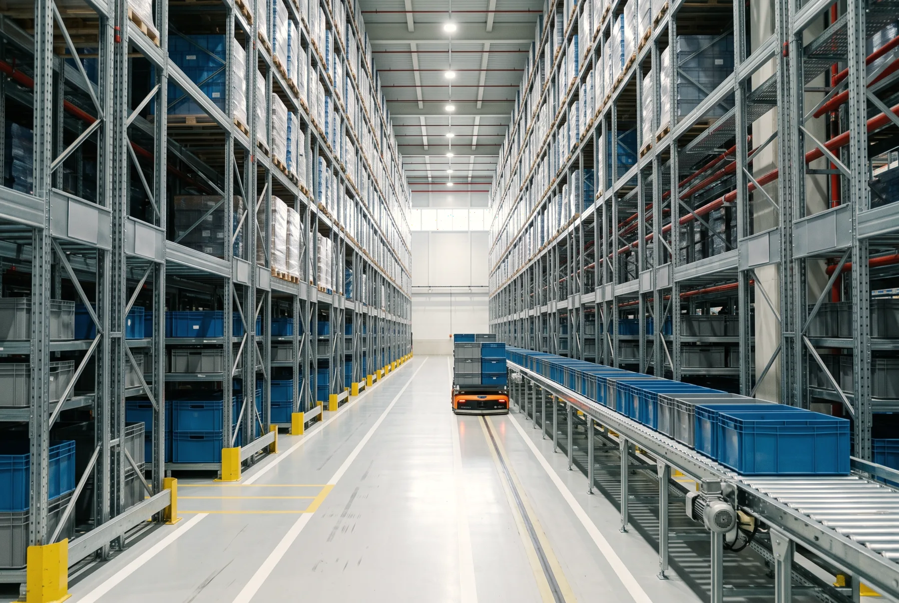
An aisle inside an automated warehouse, high-bay racking either side and painted floor guidance lines
AI-generated illustration

Scheduling here is routinely reduced to a single metric — turnover rate, or shortest path. The real cost structure is considerably richer: horizontal travel and vertical lift draw very different amounts of power, tariffs vary by time of day, shared hardware across tenants means maintenance has to dodge each tenant's own peak, and some goods add hard temperature and delivery-window constraints on top.

A schedule optimised for one metric pays the difference back somewhere unmeasured. Path length saved can reappear as contracted capacity pressure at peak. Delivery time compressed can reappear as fuel burned in detours and idling.

What we work on is turning things normally treated as fixed overhead into scheduling variables — energy, idle vehicles, idle equipment, the physical properties of a storage location. Conventional warehouse management and fleet dispatch systems do not reach this layer, and it is usually where the remaining headroom on existing hardware actually is.

Case 01Automated warehousing

Warehouse scheduling that balances SLA, throughput and energy cost

Scheduling a large automated warehouse on turnover alone ignores how much equipment dynamics and tariff structure move the actual cost.

-24%Peak-season system electricity cost
-22%Equipment travel distance
-13%Access (I/O) cycle time

The problem

We led the control-system design for a large automated storage and retrieval facility. Compared with a simple warehouse, it had many dynamic access points, equipment shared across tenants, wide variation in the physical energy cost of each movement, and goods with awkward handling properties.

The brief was to hold a strict SLA while maximising operational efficiency and minimising energy cost — three goals that conventional scheduling logic tends to trade off against each other.
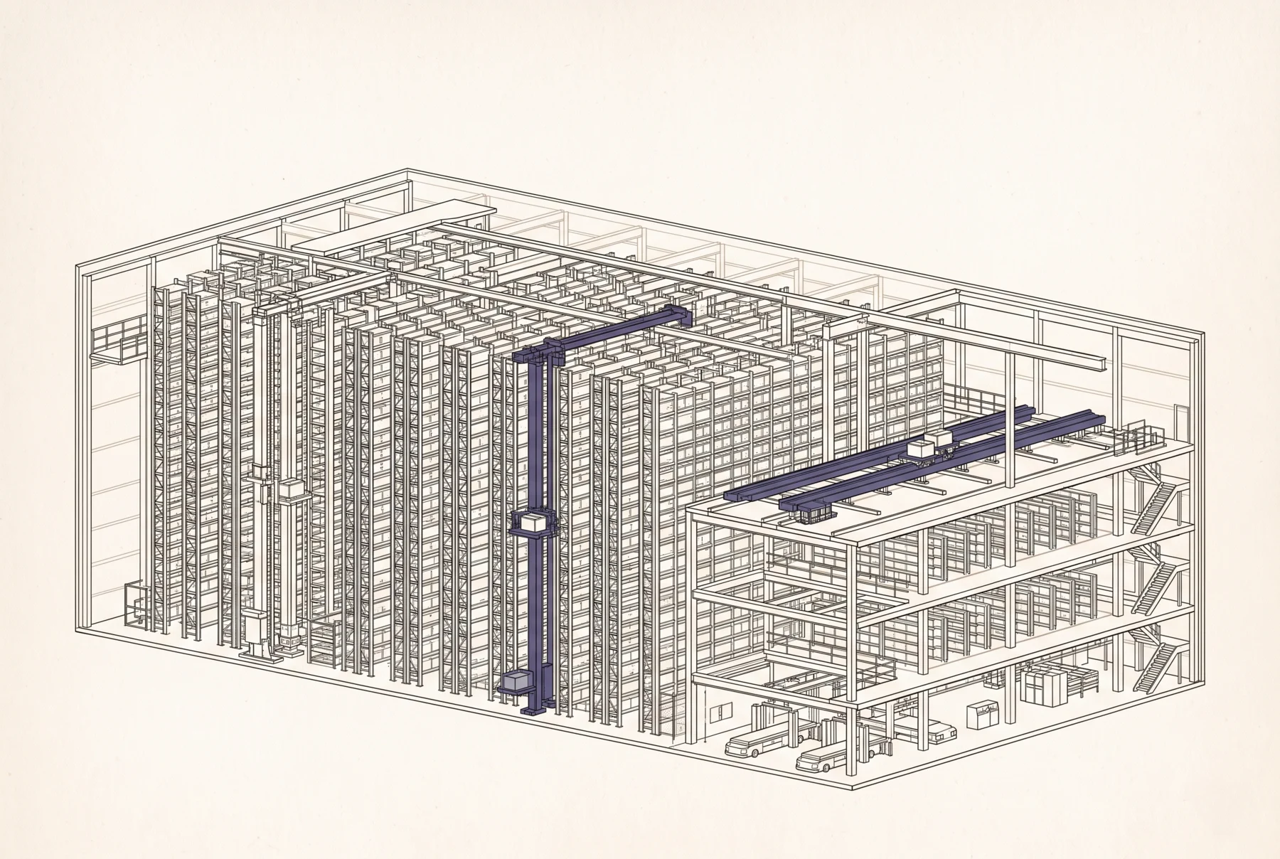
Cutaway of an automated storage facility showing stacked storage levels, vertical lift mechanisms, horizontal shuttles and multiple access nodes
An AS/RS with multiple dynamic access nodes. The difference in energy cost between vertical lift and horizontal travel is one of the scheduler's primary inputs.AI-generated illustration
Energy is not a fixed overhead. It is a variable the scheduler can actively optimise.

What we built

  1. 01
    An energy and path optimisation modelRather than ranking slots by turnover, we built an energy model incorporating the drive characteristics of the equipment, measuring the real difference between horizontal travel and vertical lift, and replacing a single reference point with multiple dynamic access nodes so every retrieval picks the lowest-energy, shortest-path slot.
  2. 02
    Off-peak tariff arbitrage and overnight stagingTime-of-use pricing is written into the scheduler. Overnight, when tariffs are lowest and equipment is idle, pallets for the next day are moved to staging, cutting daytime peak demand and contracted capacity pressure while speeding up the morning shift.
  3. 03
    Multi-tenant SLA protection and predictive maintenanceMaintenance windows are scheduled against each tenant's historical inbound and outbound peaks, so servicing shared hardware never lands on someone's busiest hours.
  4. 04
    Physical exclusion constraintsGoods carry physical and chemical property tags; strongly aromatic items and odour-absorbing items are kept apart by a dynamic safety-distance rule, so the optimiser never trades storage quality for a shorter path.
  5. 05
    Elastic capacity and yield managementBorrowing from cloud resource scheduling, the system continuously computes tenant throughput and seasonality, releasing surplus reserved slots for existing customers to expand into at peak, or offering idle capacity to the market on short high-rate terms.
TariffOff-peakMid-peakPeakMid-peakBeforeAfterOvernight stagingPeak shaved0006121824
Time-of-use pricing written into the scheduler: staging happens overnight when tariffs are lowest and equipment is idle, cutting both daytime peak draw and contracted capacity pressure.

The business case

Higher yield per square metre and better operating margin, with no additional hardware investment.

Once a scheduler can reason about energy, the ceiling on what the same hardware can return is redrawn — a layer conventional warehouse management systems do not touch.

Case 02Logistics · Distribution

Urban delivery fleets: demand forecasting, dynamic routing and order consolidation

B2B ordering patterns vary sharply in both frequency and size, and dispatch built on manual planning and driver experience could not carry the growth.

100% → 146%Distance delivered per unit of fuel (two months cumulative)
-23%Fuel use per driver, first month
-11%Fuel use per driver, a further drop in month two

The problem

A B2B urban distribution provider. Traffic conditions were complex and B2B customers varied widely in how often and how much they ordered, so dispatch based on manual planning and driver experience could not keep up with growth.

Late deliveries
Traffic and load/unload times were hard to predict, arrival windows were unreliable, and the receiving end had its own day disrupted in turn.
Unbalanced capacity
Without order forecasting, the fleet swung between idle vehicles and insufficient coverage.
Hidden fuel cost
Routing that ignored vehicle condition and live traffic produced wasted mileage and idling.

What we built

  1. 01
    Demand forecasting and dynamic dispatchMachine learning on each customer's transaction history predicts area-level demand, letting the control centre size the next day's capacity in advance and schedule vehicles and drivers against it.
  2. 02
    Multi-variable route optimisationLive traffic, vehicle condition, temperature-zone constraints and each driver's familiarity with an area are modelled together to compute the delivery sequence that minimises fuel while still meeting customer receiving windows.
  3. 03
    Order consolidationAt dispatch, geographically adjacent orders are assigned to the same driver so one stop serves several drops, raising delivery density.
BeforeEach driver crosses the whole area; routes overlapAfterOne stop, several drops
The same orders before and after consolidation. What changes is not only route length but the number of stops itself.
Dispatch moved from individual driver judgement to a system decision that can be reproduced and audited.

The business case

On-time delivery and fuel efficiency both improved materially after rollout.

For a logistics provider that keeps growing, whether dispatch can be reproduced and audited is what decides whether it can scale — dispatch quality held together by experience does not grow with the fleet.

Need Professional Assistance?

Our team are senior engineers and former executives with 20+ years in commercial product development — from apps serving hundreds of millions of users to B2B SaaS platforms serving tens of thousands of merchants. In recent years the focus has been enterprise AI adoption, from mapping the opportunity through to tuning what is live. Whether that means:

  • Mapping AI opportunities and sequencing them
  • Preparing data flows and integrating existing systems
  • Building forecasting and optimisation models
  • Monitoring and tuning after go-live
  • Test strategy and process review
  • Building and adopting test automation

We can provide professional advice and concrete solutions for teams of different scales and types. If you're facing similar challenges, feel free tocontact our consulting team.